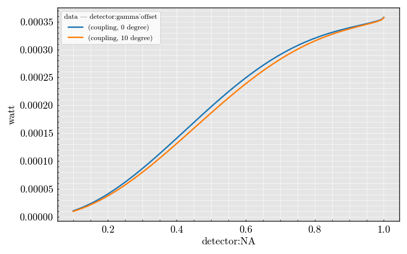
Sphere: Coupling vs numerical aperture

Importing the package dependencies: numpy, PyMieSim

import numpy as np
from TypedUnit import ureg
from PyOptik import Material

from PyMieSim import experiment
from PyMieSim import single

Defining the source to be employed.

source = experiment.source.Gaussian(
    wavelength=500 * ureg.nanometer,
    polarization=0 * ureg.degree,
    optical_power=1e-3 * ureg.watt,
    NA=0.2 * ureg.AU,
)

Defining the ranging parameters for the scatterer distribution

scatterer = experiment.scatterer.Sphere(
    diameter=500e-9 * ureg.meter,
    property=Material.BK7,
    medium_property=1 * ureg.RIU,
    source=source,
)

Defining the detector to be employed.

detector = experiment.detector.Photodiode(
    NA=np.linspace(0.1, 1, 150) * ureg.AU,
    phi_offset=0 * ureg.degree,
    gamma_offset=[0, 10] * ureg.degree,
    sampling=2000 * ureg.AU,
)

Defining the experiment setup

setup = experiment.Setup(scatterer=scatterer, source=source, detector=detector)

Measuring the properties

dataframe = setup.get("coupling", drop_unique_level=True)

Plotting the results

dataframe.plot(x="detector:NA")

single_source = single.Gaussian(
    wavelength=950 * ureg.nanometer,
    polarization=0 * ureg.degree,
    optical_power=1e-3 * ureg.watt,
    NA=0.2 * ureg.AU,
)

single_scatterer = single.scatterer.Sphere(
    diameter=500 * ureg.nanometer,
    property=Material.BK7,
    medium_property=1 * ureg.RIU,
    source=single_source,
)


print(single_scatterer.Qsca * 1e-3)

0.0010531644483825241 dimensionless