Far-Fields Computation and Visualization

This example demonstrates the process of computing and visualizing the far-fields of a scatterer using PyMieSim.

• 
• 
• 

from PyMieSim.units import ureg
from PyMieSim.single.source import Gaussian
from PyMieSim.polarization import PolarizationState
from PyMieSim.single.scatterer import Sphere
from PyMieSim.single.setup import Setup

polarization = PolarizationState(angle=30 * ureg.degree)

source = Gaussian(
    wavelength=1000 * ureg.nanometer,
    polarization=polarization,
    optical_power=1 * ureg.watt,
    numerical_aperture=0.3,
)

scatterer = Sphere(
    diameter=1500 * ureg.nanometer,
    material=1.4,
    medium=1.0,
)

setup = Setup(
    scatterer=scatterer,
    source=source,
)

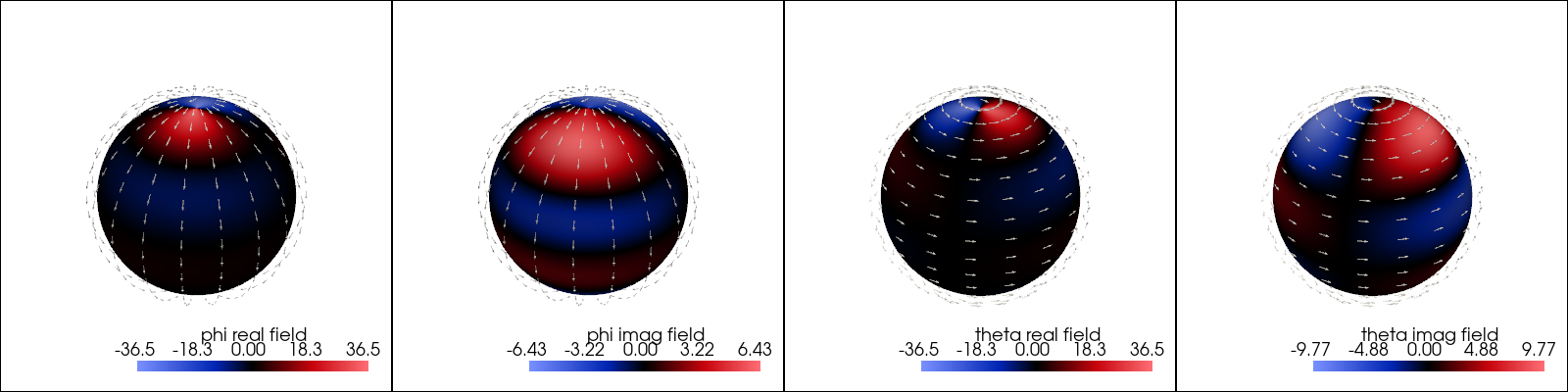
far_fields = setup.get_representation("farfields", sampling=100)

## Visualize the far-fields: phi_real component
figure = far_fields.plot("phi_real")

## Visualize the far-fields: phi_imag component
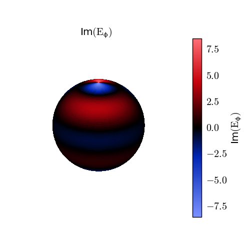
figure = far_fields.plot("phi_imag")

## Visualize the far-fields: phi_magnitude component
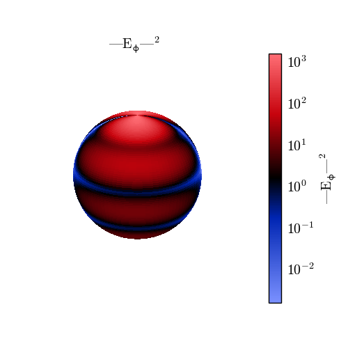
figure = far_fields.plot("phi_intensity")