How distribution width changes the scattering phase function

Compare lognormal number distributions at the same median diameter. The right panel shows the unpolarized phase function per unit solid angle, normalized so its integral over the sphere is one. Intensities are averaged before normalization; averaging complex amplitudes or equally weighted normalized single-particle phase functions would give a different result.

diameter_sampling controls the number of diameter quadrature nodes, not the number of physical particles. angular_sampling independently controls the resolution of the plotted scattering angles. Increase diameter sampling to check convergence of the ensemble phase function.

This uses the non-interacting approximation: no interparticle electromagnetic coupling, multiple scattering, or interparticle interference. Refer to PackLab for correlation-based dependent-scattering approximations when correlations matter. The comparison isolates width at fixed number median; the arithmetic mean diameter and particle volume therefore also change with width.

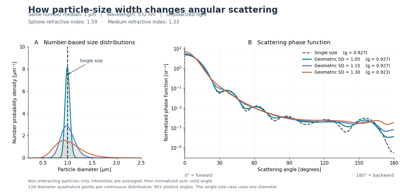
import matplotlib.pyplot as plt
import numpy as np

from PyMieSim import Measure, ParticleSizeDistribution, PlaneWave, PolarizationState, Simulation, Sphere, ureg


MEDIAN_DIAMETER = 1.0 * ureg.micrometer
WAVELENGTH = 532 * ureg.nanometer
PARTICLE_INDEX = 1.59
MEDIUM_INDEX = 1.33
WIDTHS = (1.0, 1.05, 1.15, 1.30)
DIAMETER_SAMPLING = 128
ANGULAR_SAMPLING = 901


def ensemble_phase_function(distribution, angles):
    """Return an incoherent, normalized unpolarized phase function and mean g.

    The two orthogonal polarization intensities are averaged for each sphere.
    All diameters share wavelength and medium, so the common amplitude scale
    cancels during normalization. Gauss-Legendre angular integration checks
    the normalization independently of the displayed angular grid.
    """
    source = PlaneWave(
        wavelength=WAVELENGTH, amplitude=1 * ureg.volt / ureg.meter,
        polarization=PolarizationState(angle=0 * ureg.degree),
    )
    cosine, angular_weights = np.polynomial.legendre.leggauss(512)
    evaluation_angles = np.concatenate([angles, np.arccos(cosine)]) * ureg.radian
    mean_intensity = np.zeros(len(evaluation_angles))
    scattering_weights = []
    asymmetries = []
    for diameter, fraction in zip(distribution.diameters, distribution.number_fractions):
        simulation = Simulation(
            source=source,
            scatterer=Sphere(diameter=diameter, material=PARTICLE_INDEX, medium=MEDIUM_INDEX),
        )
        s1, s2 = simulation.get_s1s2(evaluation_angles)
        intensity = (np.abs(s1.magnitude) ** 2 + np.abs(s2.magnitude) ** 2) / 2
        mean_intensity += fraction * intensity
        scattering_weights.append(fraction * simulation.run(Measure.CSCA).magnitude)
        asymmetries.append(simulation.run(Measure.G).magnitude)

    integrated = mean_intensity[len(angles):]
    normalization = 2 * np.pi * np.dot(angular_weights, integrated)
    phase = mean_intensity[:len(angles)] / normalization
    g_from_angles = 2 * np.pi * np.dot(angular_weights, cosine * integrated) / normalization
    g_from_cross_sections = np.dot(scattering_weights, asymmetries) / np.sum(scattering_weights)
    np.testing.assert_allclose(g_from_angles, g_from_cross_sections, atol=2e-7, rtol=0)
    # The unscaled angular integral must agree with the Mie scattering cross
    # section up to the common wavenumber-squared factor for all diameters.
    wavenumber = 2 * np.pi * MEDIUM_INDEX / WAVELENGTH.to('meter').magnitude
    np.testing.assert_allclose(normalization / wavenumber ** 2, np.sum(scattering_weights), rtol=2e-7, atol=0)
    return phase, g_from_angles


def make_figure(diameter_sampling=DIAMETER_SAMPLING, angular_sampling=ANGULAR_SAMPLING):
    """Plot the number distributions and their ensemble phase functions."""
    angles = np.linspace(0, np.pi, angular_sampling)
    diameters_um = np.linspace(0.2, 2.5, 1000)
    colors = ('#253449', '#007f86', '#4676c4', '#d26435')
    phase_functions = []
    with plt.rc_context({'font.size': 11, 'axes.spines.top': False, 'axes.spines.right': False}):
        figure, (size_axis, phase_axis) = plt.subplots(
            1, 2, figsize=(13, 6.3), gridspec_kw={'width_ratios': [1, 1.85]},
        )
        figure.subplots_adjust(left=0.07, right=0.98, bottom=0.19, top=0.76, wspace=0.27)
        figure.suptitle('How particle-size width changes angular scattering', x=0.07, y=0.97,
                         ha='left', fontsize=20, fontweight='bold', color='#253449')
        figure.text(0.07, 0.88,
                    'Same number median: 1 µm   |   Wavelength: 532 nm   |   Unpolarized light\n'
                    'Sphere refractive index: 1.59   ·   Medium refractive index: 1.33',
                    color='#526071', linespacing=1.6)

        for width, color in zip(WIDTHS, colors):
            distribution = ParticleSizeDistribution.lognormal(MEDIAN_DIAMETER, width, sampling=diameter_sampling)
            phase, asymmetry = ensemble_phase_function(distribution, angles)
            phase_functions.append(phase)
            if width == 1:
                label = 'Single size'
                size_axis.axvline(1, color=color, linewidth=2, linestyle='--')
                size_axis.annotate('Single size', xy=(1, 7.5), xytext=(1.25, 8.6), color=color,
                                   arrowprops={'arrowstyle': '->', 'color': color}, fontsize=10)
            else:
                label = f'Geometric SD = {width:.2f}'
                sigma = np.log(width)
                density = np.exp(-0.5 * (np.log(diameters_um) / sigma) ** 2) / (diameters_um * sigma * np.sqrt(2 * np.pi))
                size_axis.plot(diameters_um, density, color=color, linewidth=2)
                size_axis.fill_between(diameters_um, density, color=color, alpha=0.09)
            phase_axis.semilogy(np.rad2deg(angles), phase, color=color, linewidth=1.8 if width == 1 else 2.3,
                                linestyle='--' if width == 1 else '-', label=f'{label}    (g = {asymmetry:.3f})')

        size_axis.set(title='A   Number-based size distributions', xlabel='Particle diameter [µm]',
                      ylabel='Number probability density [µm⁻¹]', xlim=(0.2, 2.5), ylim=(0, 10))
        phase_axis.set(title='B   Scattering phase function', xlabel='Scattering angle [degrees]',
                       ylabel='Normalized phase function [sr⁻¹]', xlim=(0, 180))
        phase_axis.set_xticks(np.arange(0, 181, 30))
        phase_axis.legend(loc='upper right', frameon=False, fontsize=10)
        phase_axis.grid(which='major', alpha=0.15)
        size_axis.grid(axis='y', alpha=0.15)
        phase_axis.text(0, -0.17, '0° = forward', transform=phase_axis.transAxes, fontsize=10, color='#526071')
        phase_axis.text(1, -0.17, '180° = backward', transform=phase_axis.transAxes, ha='right', fontsize=10, color='#526071')
        figure.text(0.07, 0.035,
                    'Non-interacting particles only. Intensities are averaged, then normalized over solid angle.\n'
                    f'{diameter_sampling} diameter quadrature points per continuous distribution; '
                    f'{angular_sampling} plotted angles. The single-size case uses one diameter.',
                    color='#526071', fontsize=9.5, linespacing=1.6)
    return figure, np.asarray(phase_functions)


figure, phase_functions = make_figure()
plt.show()