Diagnose a sphere fit across several wavelengths

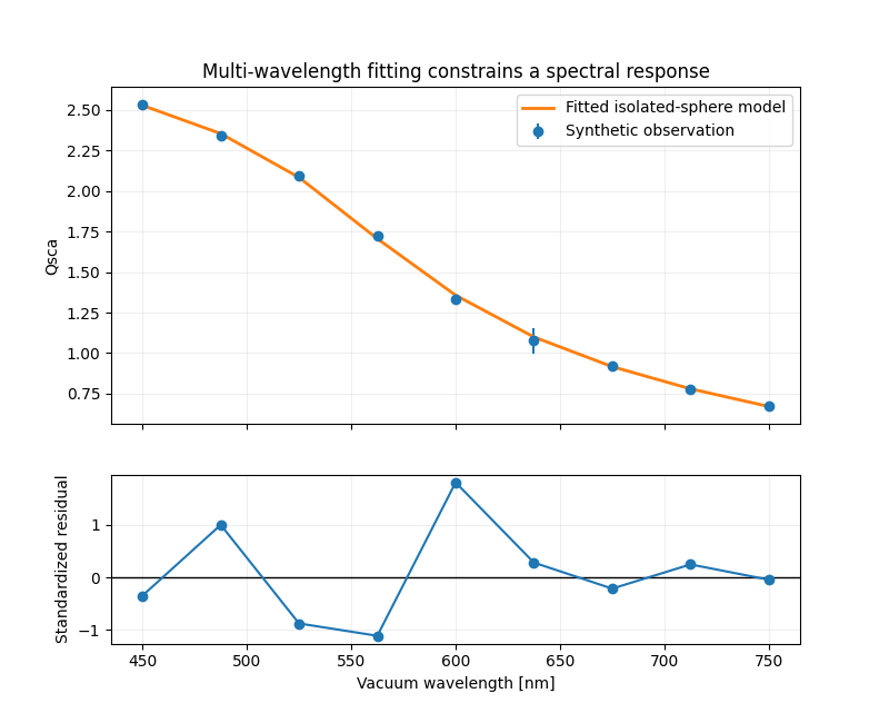
A single scattering measurement can leave diameter and refractive index ambiguous. A spectrum supplies more structure, while residuals show whether the fitted isolated-sphere model explains every channel consistently.

The synthetic observation below uses reproducible Gaussian noise and contains one deliberately biased wavelength. That channel is assigned a larger uncertainty, so it contributes less to the weighted objective. ParameterFitResult.residuals uses (prediction - observation) / uncertainty; a point above the model therefore has a negative standardized residual.

converged (614 model evaluations)
objective = 6.552419
{'diameter': <Quantity(309.803009, 'nanometer')>, 'refractive_index': 1.580155029296874}
Standardized residual shape: (9,)

import matplotlib.pyplot as plt
import numpy as np

from PyMieSim import Measure, FitParameter, MeasuredData, PlaneWave, PolarizationState, Simulation, Sphere, fit_parameters, ureg

wavelengths = np.linspace(450, 750, 9) * ureg.nanometer


def scattering_spectrum(diameter, refractive_index):
    """Return isolated-sphere scattering efficiencies at all wavelengths."""
    spectrum = np.empty(wavelengths.size)
    for index, wavelength in enumerate(wavelengths):
        source = PlaneWave(
            wavelength=wavelength,
            polarization=PolarizationState(angle=0 * ureg.degree),
            amplitude=1 * ureg.volt / ureg.meter,
        )
        simulation = Simulation(
            scatterer=Sphere(
                diameter=diameter,
                material=refractive_index,
                medium=1.0,
            ),
            source=source,
        )
        spectrum[index] = simulation.get(Measure.QSCA).magnitude
    return spectrum


observed = scattering_spectrum(
    diameter=310 * ureg.nanometer,
    refractive_index=1.58,
)
uncertainty = np.full_like(observed, 0.015)
uncertainty[5] = 0.08
rng = np.random.default_rng(seed=42)
observed = observed + rng.normal(loc=0.0, scale=uncertainty)
observed[5] += 0.08


def model(parameters):
    return scattering_spectrum(
        diameter=parameters["diameter"],
        refractive_index=parameters["refractive_index"],
    )


result = fit_parameters(
    model=model,
    observation=MeasuredData(values=observed, uncertainty=uncertainty),
    parameters=[
        FitParameter(
            name="diameter",
            initial=240 * ureg.nanometer,
            bounds=(150 * ureg.nanometer, 450 * ureg.nanometer),
        ),
        FitParameter(name="refractive_index", initial=1.45, bounds=(1.2, 2.0)),
    ],
)

print(result.summary())
print(result.parameters)
print("Standardized residual shape:", result.residuals.shape)  # (9,)

wavelength_values = wavelengths.to("nanometer").magnitude
figure, axes = plt.subplots(2, 1, figsize=(8, 6.5), sharex=True, height_ratios=(2, 1))
axes[0].errorbar(wavelength_values, observed, yerr=uncertainty, fmt="o", label="Synthetic observation")
axes[0].plot(wavelength_values, result.prediction, linewidth=2, label="Fitted isolated-sphere model")
axes[0].set(ylabel="Qsca", title="Multi-wavelength fitting constrains a spectral response")
axes[0].legend()
axes[1].axhline(0, color="black", linewidth=1)
axes[1].plot(wavelength_values, result.residuals, "o-")
axes[1].set(xlabel="Vacuum wavelength [nm]", ylabel="Standardized residual")
for axis in axes:
    axis.grid(alpha=0.2)
plt.show()