Separate scattering and absorption resonances

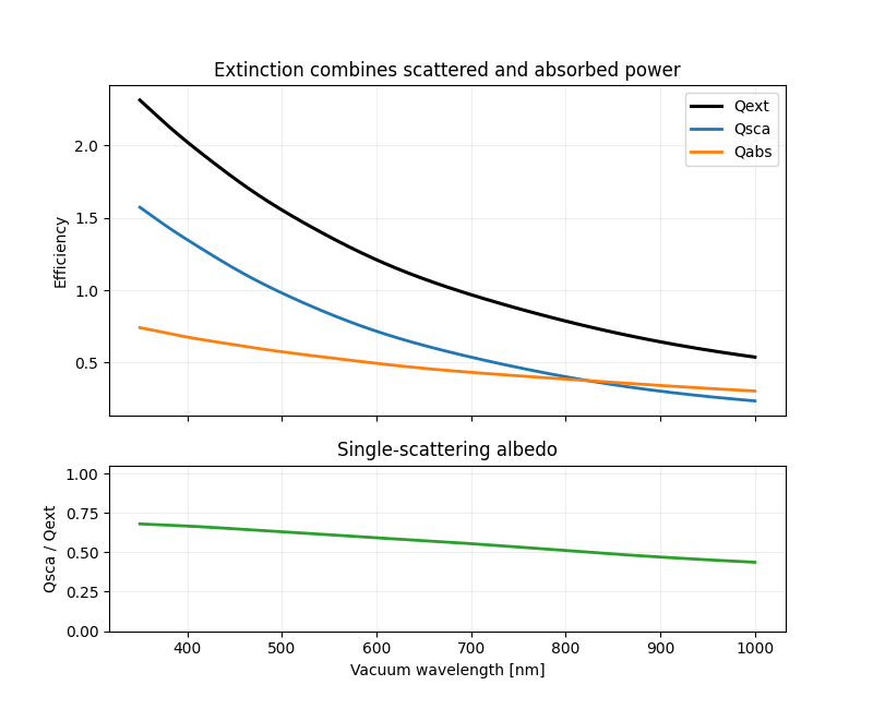
A peak in extinction does not by itself say where the removed incident power goes. This wavelength scan separates Qext into Qsca and Qabs for a lossy sphere. The lower panel shows the single-scattering albedo Qsca / Qext: values near one indicate that extinction is dominated by scattering, while lower values indicate a larger absorbed fraction.

The calculation concerns one isolated sphere. Peak locations depend on the particle size, complex refractive index, surrounding medium, and any material dispersion included in the model.

import matplotlib.pyplot as plt
import numpy as np

from PyMieSim import Measure, PlaneWave, PolarizationState, Simulation, Sphere, ureg

wavelengths = np.linspace(350, 1000, 260)
qsca = np.empty_like(wavelengths)
qabs = np.empty_like(wavelengths)
qext = np.empty_like(wavelengths)

for index, wavelength in enumerate(wavelengths):
    source = PlaneWave(
        wavelength=wavelength * ureg.nanometer,
        polarization=PolarizationState(angle=0 * ureg.degree),
        amplitude=1 * ureg.volt / ureg.meter,
    )
    simulation = Simulation(
        scatterer=Sphere(
            diameter=420 * ureg.nanometer,
            material=1.65 + 0.08j,
            medium=1.33,
        ),
        source=source,
    )
    measures = simulation.get(Measure.QSCA, Measure.QABS, Measure.QEXT)
    qsca[index] = measures["Qsca"].magnitude
    qabs[index] = measures["Qabs"].magnitude
    qext[index] = measures["Qext"].magnitude

single_scattering_albedo = qsca / qext

figure, axes = plt.subplots(2, 1, figsize=(8, 6.5), sharex=True, height_ratios=(2, 1))
axes[0].plot(wavelengths, qext, color="black", linewidth=2.2, label="Qext")
axes[0].plot(wavelengths, qsca, linewidth=2, label="Qsca")
axes[0].plot(wavelengths, qabs, linewidth=2, label="Qabs")
axes[0].set(ylabel="Efficiency", title="Extinction combines scattered and absorbed power")
axes[0].legend()
axes[1].plot(wavelengths, single_scattering_albedo, color="tab:green", linewidth=2)
axes[1].set(
    xlabel="Vacuum wavelength [nm]",
    ylabel="Qsca / Qext",
    ylim=(0, 1.05),
    title="Single-scattering albedo",
)
for axis in axes:
    axis.grid(alpha=0.2)
plt.show()