See how particle size reshapes angular scattering

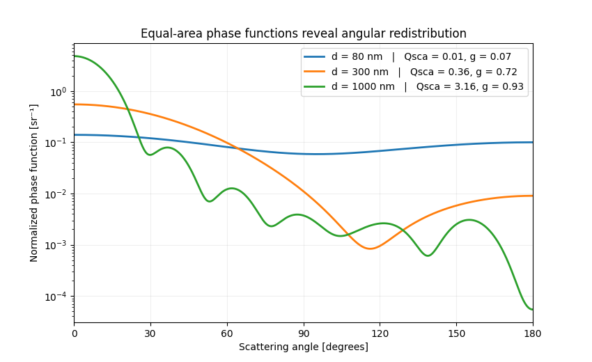
Total scattering efficiency cannot describe where the scattered power goes. This example compares normalized unpolarized phase functions for three sphere diameters at the same wavelength. As the size parameter increases, the forward lobe narrows and the angular pattern develops more structure.

Each curve integrates to one over solid angle, so the plot compares angular redistribution rather than total scattered power. The legend also reports Qsca and the asymmetry factor g to retain both pieces of information.

import matplotlib.pyplot as plt
import numpy as np

from PyMieSim import Measure, PlaneWave, PolarizationState, Simulation, Sphere, ureg

wavelength = 532 * ureg.nanometer
angles = np.linspace(0, np.pi, 1201)
source = PlaneWave(
    wavelength=wavelength,
    polarization=PolarizationState(angle=0 * ureg.degree),
    amplitude=1 * ureg.volt / ureg.meter,
)

figure, axis = plt.subplots(figsize=(8.5, 5.2))
for diameter in (80, 300, 1000):
    simulation = Simulation(
        scatterer=Sphere(
            diameter=diameter * ureg.nanometer,
            material=1.59,
            medium=1.33,
        ),
        source=source,
    )
    s1, s2 = simulation.get_s1s2(angles=angles * ureg.radian)
    intensity = (np.abs(s1.magnitude) ** 2 + np.abs(s2.magnitude) ** 2) / 2
    normalization = 2 * np.pi * np.trapezoid(intensity * np.sin(angles), angles)
    phase_function = intensity / normalization
    qsca = simulation.get(Measure.QSCA).magnitude
    asymmetry = simulation.get(Measure.G).magnitude
    axis.semilogy(
        np.rad2deg(angles),
        phase_function,
        linewidth=2,
        label=f"d = {diameter} nm   |   Qsca = {qsca:.2f}, g = {asymmetry:.2f}",
    )

axis.set(
    xlabel="Scattering angle [degrees]",
    ylabel="Normalized phase function [sr⁻¹]",
    xlim=(0, 180),
    title="Equal-area phase functions reveal angular redistribution",
)
axis.set_xticks(np.arange(0, 181, 30))
axis.grid(alpha=0.2)
axis.legend()
plt.show()